I have an Excel spreadsheet which has a column called versions. I am trying to display the version number outside of the pie chart and display a breakdown of the different version number counts in the pie chart. Can anyone help me out with this?
Good afternoon,
I think I was able to create what you are wanting. I created a google spreadsheet based on my interpretation of what you described, and linked that data. Then I used conditional formatting and dynamic shapes with formulas to get the outcome it sounds like you are describing. I used the FIELDLOOKUP formula in both the conditional formatting and the dynamic shape data field. Here are some screenshots/instructions of how I set that up. Let me know if this is what you had in mind.
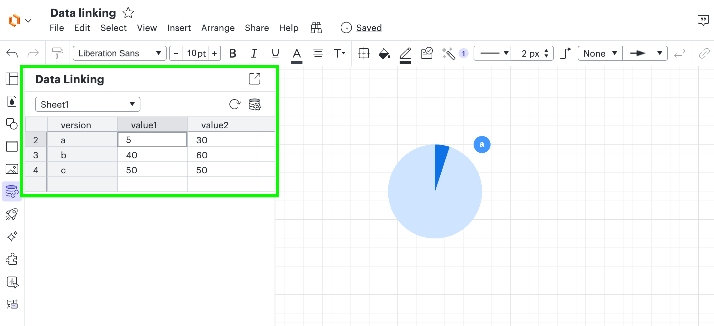
Here is what my data set looks like:

Then I added a dynamic shape (in this case I searched the shapes for “pie chart” and it showed me the dynamic shape library which I picked the pie chart from that library).
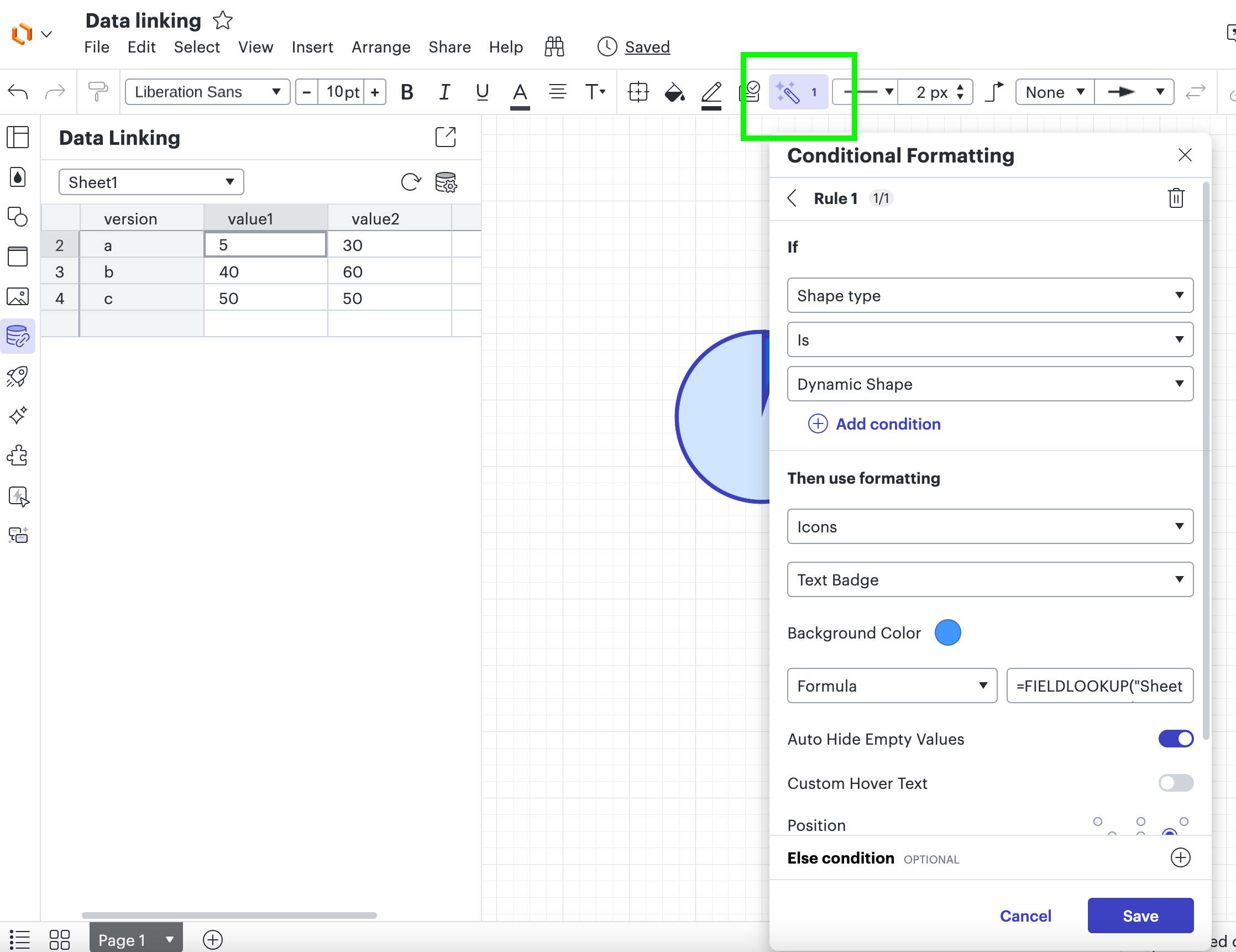
Next I went to conditional formatting and created a rule (see screenshot for the settings I used to get the badge icon to reference the version) with this formula:
=FIELDLOOKUP("Sheet1", "version", "a")
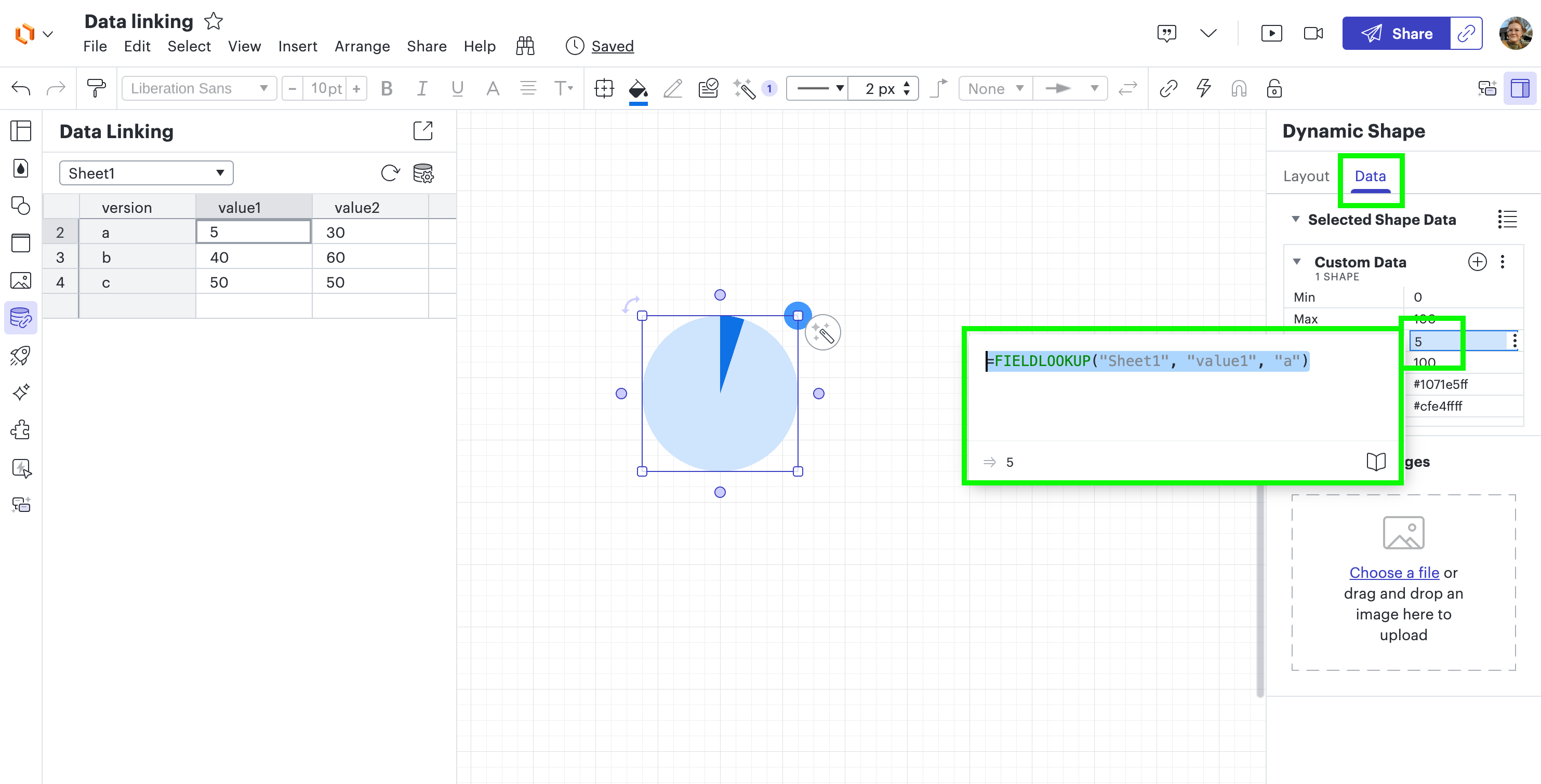
Then I used a similar formula within the dynamic shape to reference my data set. I started by selecting my dynamic shape (pie chart) then in the right hand panel clicked on data, then in the data set reflected I clicked on the “value” field and typed the equal sign (=) to begin entering a formula. The following is the formula I added to reference my data set. (see screenshot for reference as well).
=FIELDLOOKUP("Sheet1", "value1", "a")
I hope this is what you were looking for!
Reply
Create an account in the community
A Lucid account is required to interact with the community. You will be redirected to the Lucid app to create an account.
Log in to the community
A Lucid account is required to interact with the community. You will be redirected to the Lucid app to log in.
Log in with Lucid
Enter your E-mail address. We'll send you an e-mail with instructions to reset your password.