
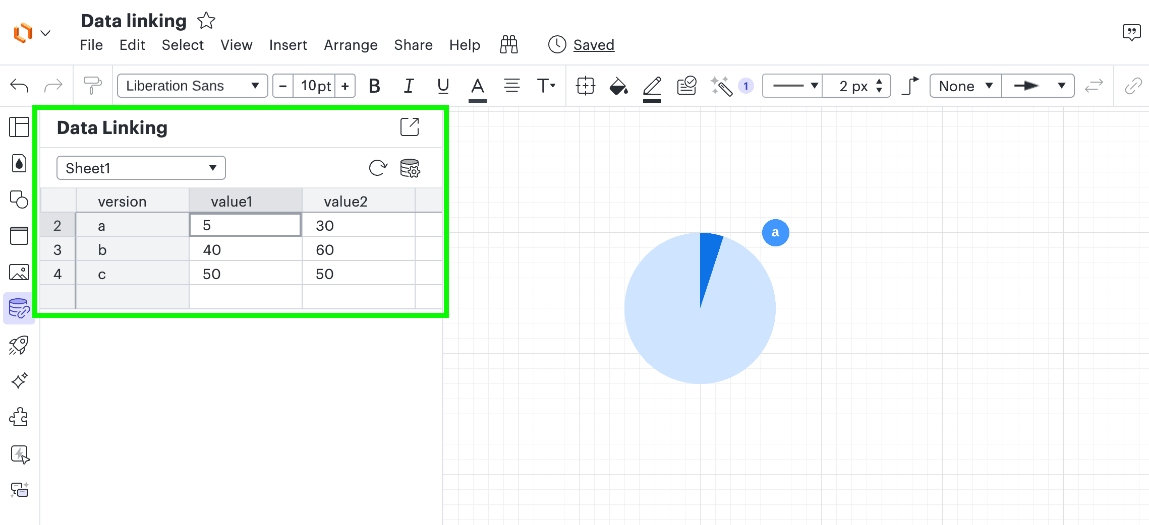
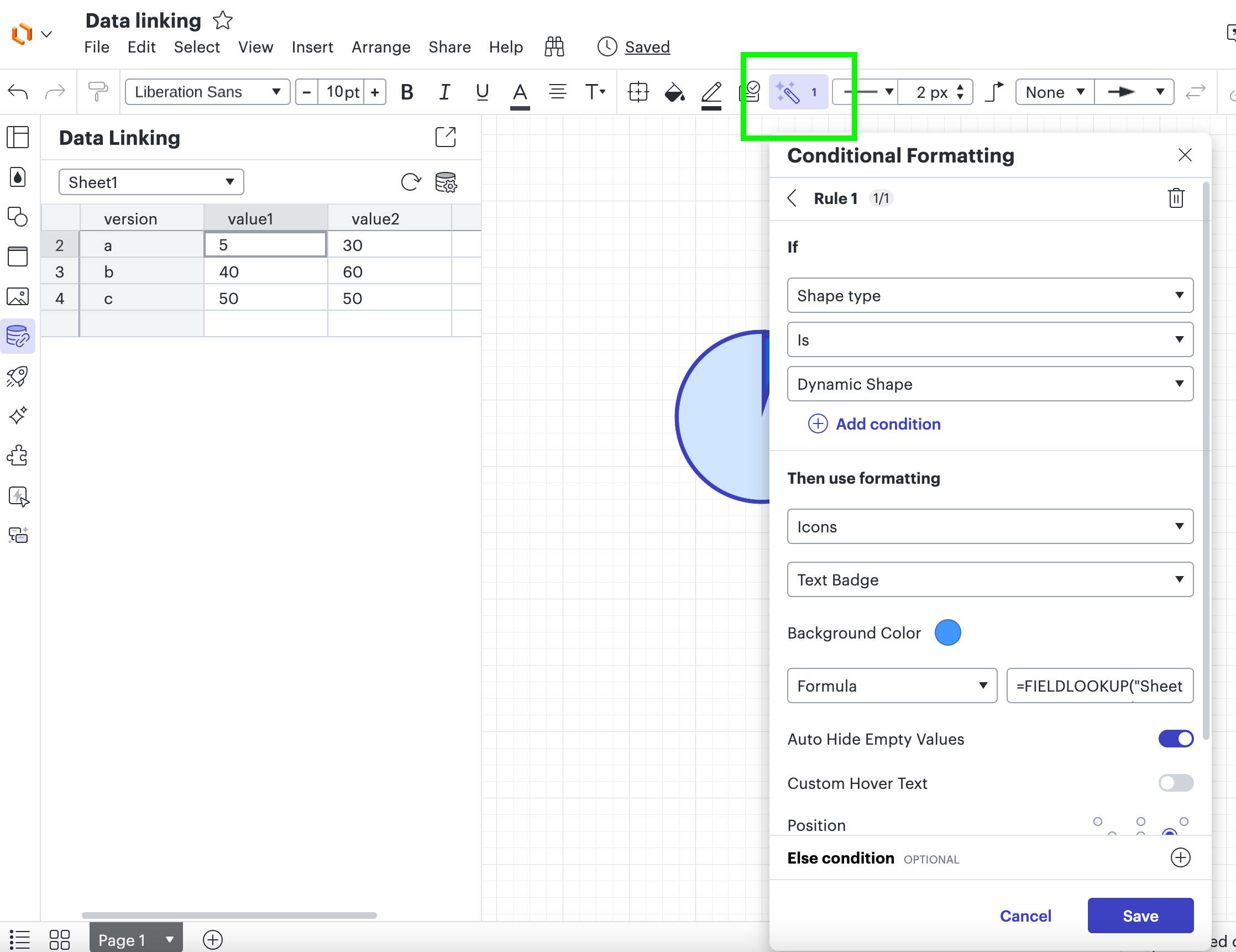
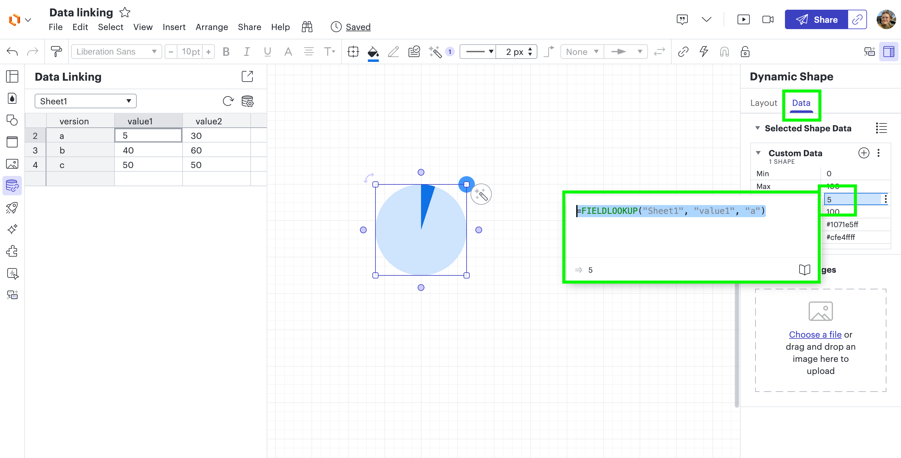
I have an Excel spreadsheet which has a column called versions. I am trying to display the version number outside of the pie chart and display a breakdown of the different version number counts in the pie chart. Can anyone help me out with this?
Question
Data Linking to Pie Chart

Create an account in the community
A Lucid or airfocus account is required to interact with the Community, and your participation is subject to the Supplemental Lucid Community Terms. You may not participate in the Community if you are under 18. You will be redirected to the Lucid or airfocus app to log in.
Log in to the community
A Lucid or airfocus account is required to interact with the Community, and your participation is subject to the Supplemental Lucid Community Terms. You may not participate in the Community if you are under 18. You will be redirected to the Lucid or airfocus app to log in.
Log in with Lucid Log in with airfocus
or
Enter your E-mail address. We'll send you an e-mail with instructions to reset your password.