Hello, 


I’m trying to create a conditional formatting rule that will highlight boxes based on the shape data I’ve linked to my diagram. I’m utilizing Google sheets to create a CSV with VLAN data for each box in our network. 


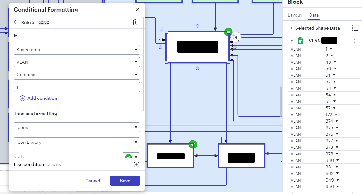
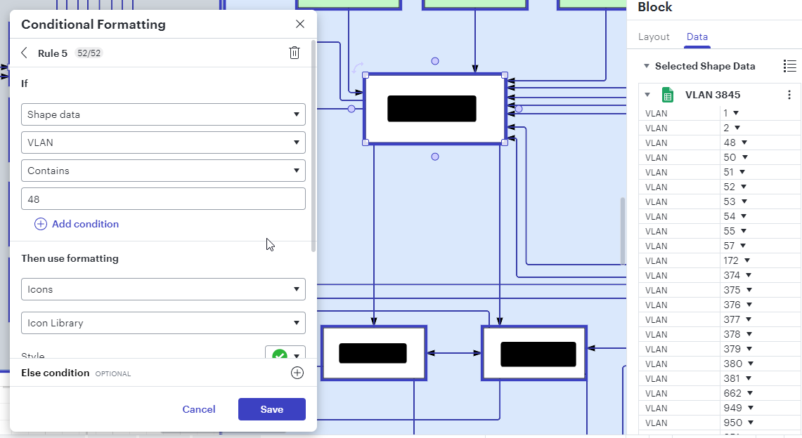
I’m unable to get the formatting to actually apply whenever I set the rule after the first column. I have attached two examples of “working” and not working. The goal is the apply the VLAN data for each box and when the rule is applied it will highlight all boxes, avoiding a lot of manual work. Maybe I’m going about this the wrong way, my Google sheets will have a tab for each box with a column header of VLAN with the numbers for that box.


Notice VLAN 1 works, but VLAN 48 does not. 


Let me know if you need additional information, thanks!

Another note, both of the boxes with green check marks are using separate datasets/sheets on my Google sheets file, so it seems to be working to a degree. 


Hi @lucidjoe

Thank you for your post! Could you try the following to steps to see if they resolve the issue?

  • Could you try force syncing your data by clicking the refresh button above where the data is shown in Lucidchart?
  • If your data still does not refresh, please try re-uploading your data using "replace data set".

If the issue persists, can you please send a temporary Support PIN for this document? This will allow me to take a closer look at the issue you’re experiencing. For more information on generating a Support PIN, check out this Help Center article.


Hi @lucidjoe

Thank you for your post! Could you try the following to steps to see if they resolve the issue?

  • Could you try force syncing your data by clicking the refresh button above where the data is shown in Lucidchart?
  • If your data still does not refresh, please try re-uploading your data using "replace data set".

If the issue persists, can you please send a temporary Support PIN for this document? This will allow me to take a closer look at the issue you’re experiencing. For more information on generating a Support PIN, check out this Help Center article.


Hi Kelsey,


I did the 2 steps you mentioned but still no luck, I have generated a support PIN. 


Can I directly message you the support PIN or create a ticket so it’s not posted publicly.


Thanks!


Hi @lucidjoe

Thank you for trying those steps! You can PM me the support pin if you feel more comfortable doing that! Just so you know, only our Support Team can activate a support pin because only we have access to the tool to use a support pin and your unique user ID.


Thanks @Kelsey Gaag ,


I have PM’d you the PIN and information on the diagram, let me know if you have any additional questions. 


Hi @lucidjoe

After taking a closer look, it looks like the reason this issue is occurring is because in your data set in the right column there are several of the same reference key, “VLAN,” so the conditional formatting is referencing the first cell.

I’m looking further into this issue and into possible solutions for this issue with our engineers.


Hi @Kelsey Gaag


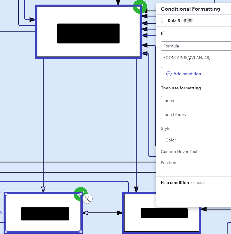
Thanks for taking a look! I may have found a solution that works. I am using the following formula:

=CONTAINS(@VLAN, 48)


Found this information from this site: https://developer.lucid.co/formulas/#references


This is what I expected from using “If > Shape Data > VLAN > Contains > 48” conditional formatting to achieve. I’ll be curious if this is a bug or intended, but I’m considering this as my solution and will mark this as solved.


Thanks for the help!


Hi @lucidjoe

Glad you were able to find a solution to this issue! The developers I was in contact with suggested a similar solution which is to use  using a COUNTIF to count how many of the VLANs have a value of 48:

=COUNTIF(this.VLAN, x => x = 48) > 0

(if that number is greater than 0, it has 48 in the list).
The other version is:

=COUNTIF(this.VLAN, x => x = 48) = 0


Please let me know if you need help with anything else.


Reply